Principles behind R programming

Today

What we’ll do today:

Principles behind functional programming in R
Defining your own functions
Anonymous functions
Making your functions purrrrr
Exercise: simulate data

What is a function anyway?

A function has three parts:

The formals() - the list of arguments that control how you call the function.
The body() - the code inside the function.
The environment() - the data structure that determines how the function finds the values associated with the names.

An example

sum_two_numbers <- function(x, y){
  x + y
}

formals(sum_two_numbers)

$x


$y

body(sum_two_numbers)

{
    x + y
}

environment(sum_two_numbers)

<environment: R_GlobalEnv>

An exception to the rule

body(sum)

NULL

There is one exception to the rule that a function has three components. Primitive functions, like sum() and [, call C code directly.

These functions exist primarily in C, not R, so their formals(), body(), and environment() return all NULL.

Functions are objects, too

sum_two_numbers <- function(x, y){
  x + y
}

More or less anything you can do with other objects (dataframes, variables, …), you can also do with functions

a_list_of_functions <- list(sum_two_numbers, mean, median)

a_list_of_functions[[1]](10,20)

[1] 30

But not quite anything:

a_data_frame_with_functions <- data.frame(functions = c(sum_two_numbers, mean, median))

Error in as.data.frame.default(x[[i]], optional = TRUE): cannot coerce class '"function"' to a data.frame

Anonymous functions

You don’t always need to give your functions a name. If you just want to do something once, there’s no need to define it first and invoke it later. You can simply create it on the fly, and forget about it again.

This is called an anonymous function.

There’s several ways to write them:

# long way
function(x,y) {x + y}

function(x,y) {x + y}

# shorthand
\(x, y) {x+y}

\(x, y) {x+y}

# purrr style
~.x + .y

~.x + .y

We’ll come back to those later.

Object of type closure is not subsettable

Maybe you’ve seen this error message before

mean[1:3]

Error in mean[1:3]: object of type 'closure' is not subsettable

This sometimes happens when we mess up R syntax, which leads to R trying to do something to a function that it cannot do (e.g., subset it).

The error message is also obscure because we rarely encounter the name “closure”. But in fact, almost all (except some core R functions) functions are of type closure.

typeof(mean)

[1] "closure"

The name closure is meant to signal that functions enclose their own environments.

Environments

R operates with a hierarchy of environments.

At the root sits the global environment. This is what you can see in the environment pane in RStudio.

Above that, R can invoke any number of nested environments. One important type of environments are package environments. Whenever you load a package, R creates an environment for that package, in which all its functions and other objects are defined.*

environment(sum_two_numbers)

<environment: R_GlobalEnv>

library(dplyr)
environment(mutate)

<environment: namespace:dplyr>

*R actually creates two environments, a package environment, and a namespace environment, see more here

Execution environments

Whenever you execute a function, R creates a temporary environment in which the function is evaluated. When the function is complete, the environment gets destroyed.

Only the output of the function is printed or assigned to an object, if you specify this.

my_fun <- function(){
  # this assignment only happens in the temporary execution environment 
  x <- 1
}

my_fun()

# even after running the function, the global environment will not know about the assignment
x

Error in eval(expr, envir, enclos): object 'x' not found

my_fun <- function(){
  x <- 1
  x
}

x <- my_fun()
x

[1] 1

A short quiz

Given what we know about environments, what is the outcome of the following code?

x <- 10
f01 <- function() {
  x <- 20
  x
}

f01()

[1] 20

What about calling x now?

[1] 10

What happens here?

x <- 10
f02 <- function(){
  y <- 5
  x + y
}
f02()

[1] 15

Lexical scoping

Scoping is the act of finding the value associated with a name.

For functions, the important thing to remember is that within a function, R will look first within the function execution environment, and then in its parent environments.

x <- 10

f01 <- function() {
  x <- 20
  x
}

# this returns 20, because x is found first in the function execution environment
f01()

[1] 20

# this returns 10, because outside of the function, R looks in the global environment
x

[1] 10

Lazy evaluation

R function arguments are lazily evaluated: they’re only evaluated when accessed.

For example, this code doesn’t generate an error because my_undefined_argument is never used:

h01 <- function(my_undefined_argument) {
  10
}
h01()

[1] 10

Lazy evaluation

This behavior is great because it allows more computationally efficient functions. It also allows funky default arguments (but maybe not a great idea do this..)

# A really weird function. Don't do this
h02 <- function(
    x = 1, 
    y = x + 1, 
    a
    ){
  a <- 5
  a + x + y
}

h02()

[1] 8

h02(x = 2)

[1] 10

When defining your own function, it’s important you keep an eye on whether you actually use the arguments you’ve defined in the function body. R won’t tell you…

… dot-dot-dot

Functions can be defined to take any number of additional unnamed arguments. This can be specified using the ... syntax.

g01 <- function(x, y, ...){
  c(x,y,...)
}

g01(1,2,3,4,5,6,7)

[1] 1 2 3 4 5 6 7

… dot-dot-dot

This is often useful when a function calls another function (called “forwarding”), or has a function as one of its arguments. The ... can be used to allow users to pass on arguments to the other function:

g02 <- function(x, ...){
  y <- c(x, 5)
  
  # additional arguments are forwarded to mean
  mean(y, ...)
}

g02(NA, na.rm = TRUE)

[1] 5

x <- list(c(1, 3, NA), c(4, NA, 6))
str(lapply(x, mean, na.rm = TRUE))

List of 2
 $ : num 2
 $ : num 5

Practice

Define a function that calculates the standard error for a vector of numbers.

Bonus 1: make it so you can specify na.rm = TRUE

Bonus 2: make it so that it gives some informative errors when given wrong input (e.g. a character value). Tip: check out the stopifnot() function, or use an if statement.

Practice - Solution

se <- function(x, na.rm = FALSE) {
  # stopifnot solution
  # stopifnot(is.numeric(x))
  
  # with an if statement
  if(!is.numeric(x)) {stop("x needs to be numeric")}
  
  std.dev <- sd(x, na.rm = na.rm)
  
  len <- if (!na.rm) {
    length(x)
  } else {
    length(x[!is.na(x)])
  }
  
  out <- std.dev / sqrt(len)
  out
}

x <- c(NA, 1, 5, 2, NA, -3)

se(x)

[1] NA

se(x, na.rm = TRUE)

[1] 1.652019

Non-standard evaluation

Disclaimer

Non-standard evaluation (also called tidy evaluation) is a tricky concept, and to be honest, I haven’t understood it fully myself.

For most things you’re likely to do with R, you probably won’t need a deep understanding of it. However, if you want to program with tidyverse functions, you will need to understand a few tricks.

To learn more, Hadley Wickham’s book Advanced R gives a good introduction

Non-standard evaluation light

How does select() know what you are talking about?

my_data <- tibble(col1 = c(1:5),
                  col2 = rnorm(5))

my_data %>% select(col2)

Tidyverse functions blur the boundary between environment variables (variables that exist within the global or function environment) and data variables (variables that exist as named columns in a dataframe).

Non-standard evaluation light

In base R, you would need to quote column names to select them.

# this does not work
my_data[col2]

Error in eval(expr, envir, enclos): object 'col2' not found

my_data["col2"]

Non-standard evaluation light

Tidyverse code works by combining code expressions (capturing the intent of a piece of code without evaluating it), with a data mask (a special object that basically turn data columns into objects).

It does this to make working with these functions more convenient for you - so that you don’t need to use "" all the time.

This however comes at a cost when you define your own functions that use tidyverse functions.

An example: defining a `grouped_mean()` function

# Let's turn this following code into a function
iris %>% 
  group_by(Species) %>% 
  summarise(mean_sep_length = mean(Sepal.Length))

grouped_mean <- function(data, grouping_var, values_var) {
  data %>% 
    group_by(grouping_var) %>% 
    summarise(mean_variable = mean(values_var))
}

grouped_mean(iris, Species, Sepal.Length)

Error in `group_by()`:
! Must group by variables found in `.data`.
✖ Column `grouping_var` is not found.

This does not work because R will try to evaluate grouping_var and values_var as data variables, but won’t find them in the dataset.

defining a `grouped_mean()` function

We need to tell R that we want use grouping_var and values_var as hybrid variables. It should first treat them as environment variables, and make them refer to whatever you assign them to. Then, they should be treated as data variables.

You can do that easily with the {{}} operator (pronounce “curly curly”, or the embracing operator)

grouped_mean2 <- function(data, grouping_var, values_var) {
  data %>% 
    group_by({{ grouping_var }}) %>% 
    summarise(mean = mean({{ values_var }}))
}

grouped_mean2(iris, Species, Sepal.Length)

A final complication

Using curly curly on the LHS of an assignment requires a special operator.

library(glue)

grouped_mean3 <- function(data, grouping_var, values_var, prefix = "avg") {
  data %>% 
    group_by({{ grouping_var }}) %>% 
    summarise("{prefix}_{{values_var}}" := mean({{values_var}}))
}

grouped_mean3(iris, Species, Sepal.Length)

This code uses glue() syntax to specify a new name for the new column. It also uses the walrus operator := for assignment. The walrus operator is necessary whenever you use {{}} on the left hand side of an assignment.

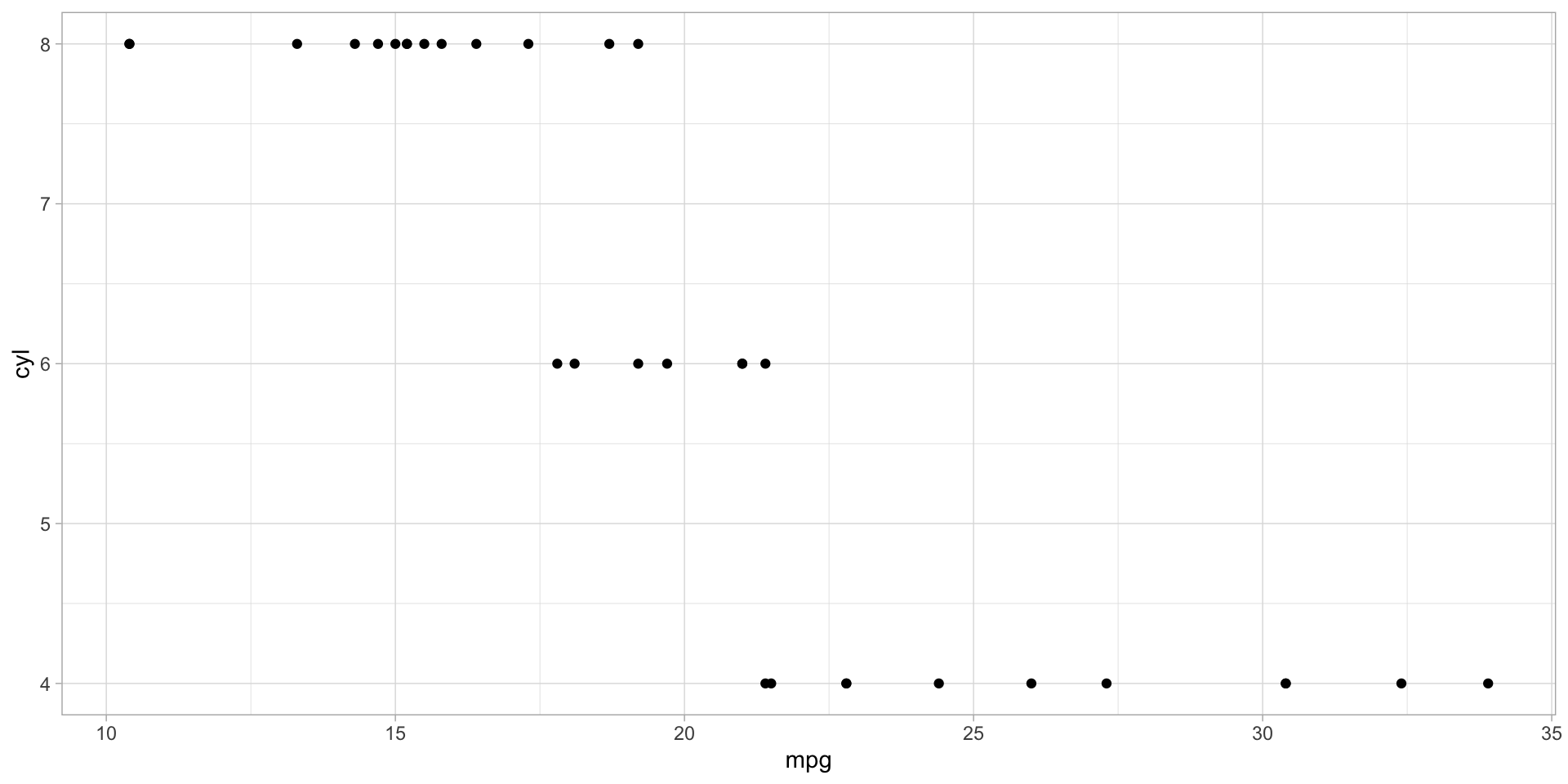
Another example: programming with ggplot

create_scatter_plot <- function(data, variable1, variable2) {
  data %>% 
    ggplot(aes(variable1, variable2)) +
    geom_point() +
    theme_light()
}

# hello darkness, my old friend
create_scatter_plot(mtcars, mpg, cyl)

Error in `geom_point()`:
! Problem while computing aesthetics.
ℹ Error occurred in the 1st layer.
Caused by error:
! object 'cyl' not found

Another example: programming with ggplot

create_scatter_plot <- function(data, variable1, variable2) {
  data %>% 
    # Curly Curly to the rescue!
    ggplot(aes({{variable1}}, {{variable2}})) +
    geom_point() +
    theme_light()
}

create_scatter_plot(mtcars, mpg, cyl)

Let’s practice

Exercise

Create a create_barchart() function that plots a bar chart of a given variable.

Bonus: make it so that bars are sorted by size (tip: use a function from the fct_ family)

Change the create_scatterplot() function so that it has a title that describes which variables are plotted.

Tip: this requires treating the name of the objects as a string. Perhaps a quick google search can help you.

Resources

Hadley Wickham’s Advanced R: https://adv-r.hadley.nz/metaprogramming.html

Principles behind R programming

Today

What we’ll do today:

What is a function anyway?

A function has three parts:

An example

An exception to the rule

Functions are objects, too

Anonymous functions

Object of type closure is not subsettable

Environments

Environments

Execution environments

A short quiz

Lexical scoping

Lazy evaluation

Lazy evaluation

… dot-dot-dot

… dot-dot-dot

Practice

Practice - Solution

Non-standard evaluation

Disclaimer

Non-standard evaluation light

Non-standard evaluation light

Non-standard evaluation light

An example: defining a grouped_mean() function

defining a grouped_mean() function

A final complication

Another example: programming with ggplot

Another example: programming with ggplot

Let’s practice

Exercise

Resources

An example: defining a `grouped_mean()` function

defining a `grouped_mean()` function