Combining Functions & Purrr for simulations

A short guide to doing simulations with purrr

A simple example

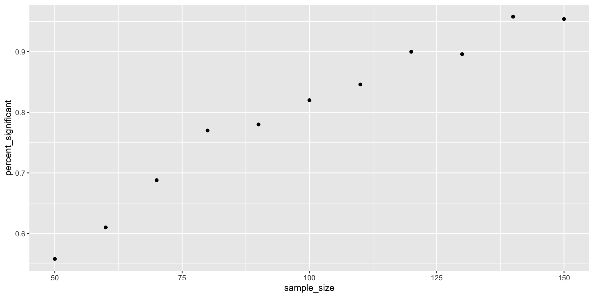
Let’s say we want to calculate the power to detect a correlation of .31

library(tidyverse)
x <- rnorm(100)
error <- rnorm(100)
y <- x * 0.3 + error

dat <- data.frame(x = x, y = y)

lm(y ~ x, data = dat) %>% 
  broom::tidy()
dat %>% 
  ggplot(aes(x,y)) +
  geom_point() +
  geom_smooth(method = "lm")

enter purrr

# Define a function that generates a random dataset
generate_data <- function(x){
  # adding the x as an argument is a bit of a hack because we don't need it
  # there's an easier way to do this in R using the replicate function
  measure_1 <- rnorm(100) 
  measure_2 <- measure_1 * 0.3 + rnorm(100)
  
  result <- data.frame(measure_1, measure_2)
}
simulations_data <- tibble(simulation_id = c(1:1000)) %>% 
  
  mutate(sim_dat = map(simulation_id, generate_data),
         model = map(sim_dat, \(x) {lm(measure_2 ~ measure_1, data = x)}),
         tidy_model = map(model, broom::tidy),
         p_value_measure_2 = map_dbl(tidy_model, \(x) x %>% 
                                       filter(term == "measure_1") %>%  
                                       pull(p.value)))
simulations_data %>% 
  summarise(power = mean(p_value_measure_2 < 0.05))

This is nice, but only for a fixed sample size…

Let’s try and make it better :)
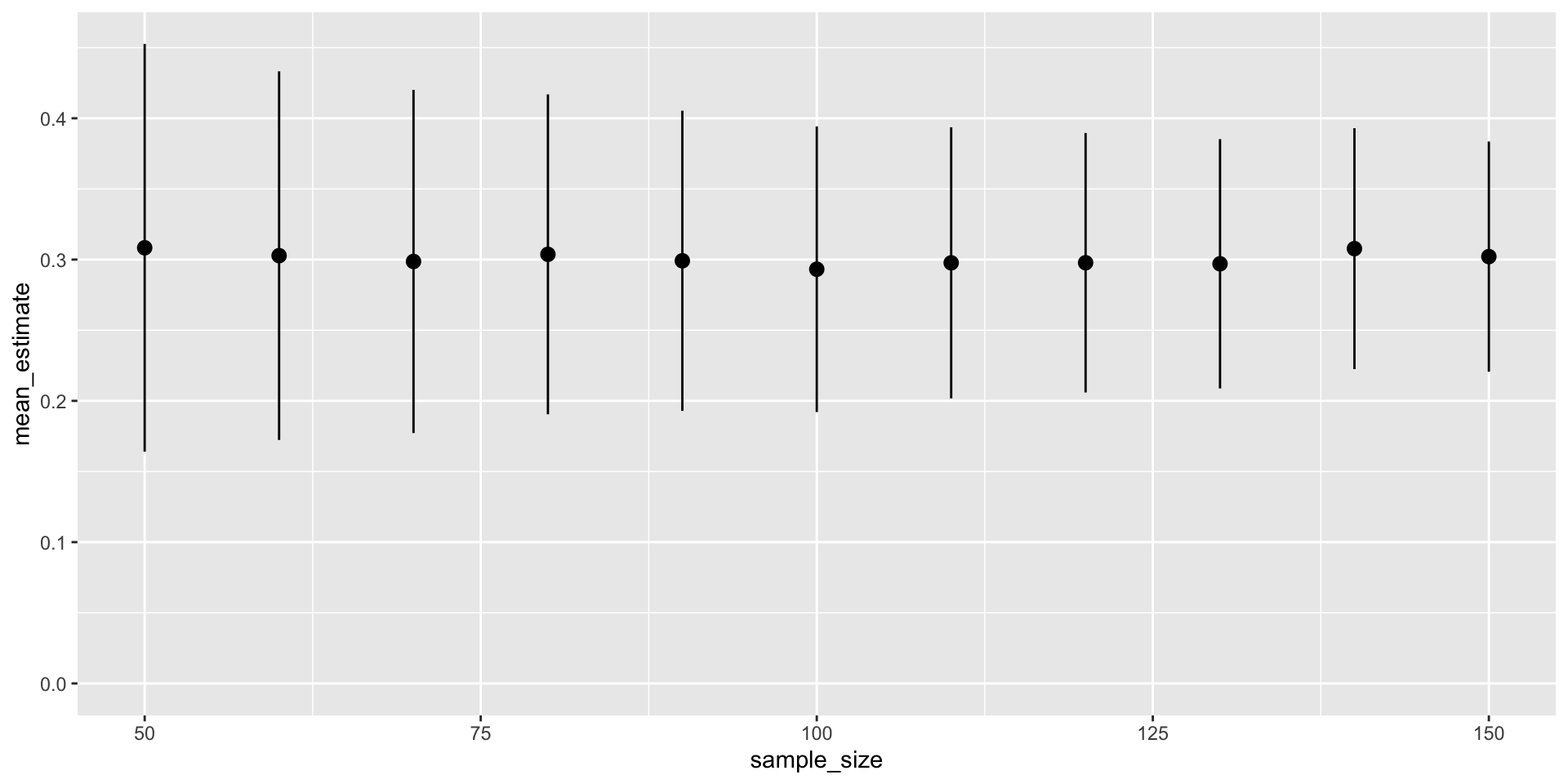
generate_data2 <- function(N){
  measure_1 <- rnorm(N) 
  measure_2 <- measure_1 * 0.3 + rnorm(N, sd = 1)
  
  result <- data.frame(measure_1, measure_2)
}
simulations_data_2 <- crossing(
  simulation_id = c(1:500),
  sample_size = seq(50, 150, by = 10)
)
sim_outcome <- simulations_data_2 %>% 
   mutate(sim_dat = map(sample_size, generate_data2),
         model = map(sim_dat, \(x) {lm(measure_2 ~ measure_1, data = x)}),
         tidy_model = map(model, broom::tidy),
         p_value_measure_2 = map_dbl(tidy_model, \(x) x %>% 
                                       filter(term == "measure_1") %>%  
                                       pull(p.value)))
sim_outcome %>% 
  group_by(sample_size) %>% 
  summarise(n_sims = n(),
            percent_significant = sum(p_value_measure_2 < 0.05) / n_sims) %>% 
  ggplot(aes(sample_size, percent_significant)) +
  geom_point()

sim_outcome %>% 
  unnest(tidy_model) %>% 
  filter(term == "measure_1") %>% 
  group_by(sample_size) %>% 
  summarise(across(c(estimate, std.error), c("mean" = mean), .names = "{.fn}_{.col}")) %>% 
  ggplot(aes(sample_size, mean_estimate, ymin = mean_estimate - mean_std.error, ymax = mean_estimate + mean_std.error)) +
  geom_pointrange() +
  expand_limits(y = c(0, 0.35))

Practice: Do the same for a t-test

Bonus: what about different effect sizes?

Resources